How to use the Excel VLOOKUP function

Simulation23 Excel Function vlookup() How To
VLOOKUP() function
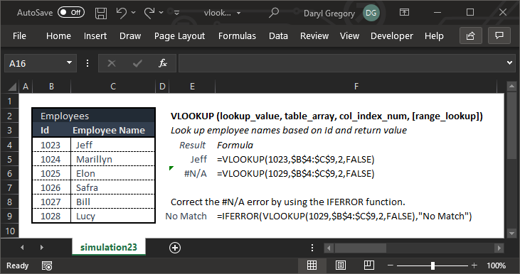
The VLOOKUP functions allows you search rows in a table for a particular value and return the value in the corresponding column specified.
HINT: When organizing your data, keep your search values on the left and the value you want to return to the right.
Syntax
VLOOKUP (lookup_value, table_array, col_index_num, [range_lookup])
- The lookup_value is the value that you are searching for and must be in the leftmost column in your table_array.
- The table_array is where you want to search for the lookup_value. The lookup_value must be the first column in the table_array. The range of the table_array must also include the return value you are searching for.
- Use the col_index_num to select the column number that contains the return value you are looking for.
- If you want to find an exact match set the range_lookup value to FALSE and for an approximate match set the value to TRUE.
Notes
- The “[ ]” brackets around the argument mean that it is optional. Beware the default value for range_lookup is TRUE.
- If you set the range_lookup value to FALSE and no match is found, the function will return a #N/A error. (To deal with the #N/A error, see the IFERROR function)
- If you plan on copying this formula from one cell to another you are going to want to set the table_array as an absolute value, which is indicated by placing dollar signs in the range.


