How to use the Excel HLOOKUP Function

Simulation23 Excel Function hlookup() How To
HLOOKUP() function
The “Horizontal Lookup” HLOOKUP function allows you search columns in a table for a particular value and return the value in the in the same column from the row specified.
Syntax
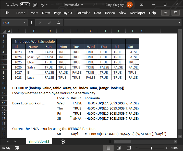
HLOOKUP (lookup_value, table_array, row_index_num, [range_lookup])
- The lookup_value is the value that you are searching for and must be in the first row of your table_array.
- The table_array is where you want to search for the lookup_value. The lookup_value must be the first row of the table_array. Values should be in ascending order, left to right.
- Use the row_index_num to select the row number that contains the return value to return.
- If you want to find an exact match set the range_lookup value to FALSE and for an approximate match set the value to TRUE.
Notes
- The “[ ]” brackets around the argument mean that it is optional. Beware the default value for range_lookup is TRUE.
- #VALUE! error occurs if the row_index_num is less than 1
- #REF! error occurs if the row_index_num is greater than the numbers of rows in the table_array.
- Use wildcard characters in the lookup_value
- Question mark, “?”, replaces a single character
- Asterisk, “*”, replaces a sequence of characters
- If you are actually searching for a question mark or asterisk, place a tilde “~” in front of the character